The price elasticity of demand calculator measures how strongly quantity demanded changes when a product’s price changes. Enter two price-and-quantity pairs to calculate elasticity using the midpoint method and compare revenue before and after the price change.

How to use the price elasticity calculator
Use observations for the same product, measured over comparable periods and under similar selling conditions.
- Initial Price: Enter the price per unit before the change.
- Initial Quantity: Enter the number of units demanded or sold at that price.
- Final Price: Enter the price per unit after the change.
- Final Quantity: Enter the number of units demanded or sold at the new price.
The calculator returns a signed price elasticity coefficient, Revenue At Initial Price, and Revenue At Final Price. The revenue figures are price multiplied by quantity—not profit.
For a meaningful comparison, use consistent units: compare units per week with units per week, not a week’s sales with a month’s sales. Use positive prices and nonnegative quantities, and keep the treatment of discounts and taxes consistent.
Price elasticity of demand formula
Price elasticity of demand divides the percentage change in quantity demanded by the percentage change in price. This calculator uses the midpoint method, also called arc elasticity, which measures each change relative to the average of its initial and final values.
PED = [(Q1 − Q0) / ((Q1 + Q0) / 2)] ÷ [(P1 − P0) / ((P1 + P0) / 2)]
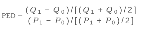
- P0: Initial price.
- P1: Final price.
- Q0: Initial quantity.
- Q1: Final quantity.
Unlike an ordinary percentage change, which uses the starting value as its base, the midpoint method uses an average. This gives the same elasticity when you reverse the initial and final observations. The percentage multipliers cancel when the two changes are divided, so the formula can use decimal changes directly.
The revenue calculations are:
- Initial revenue = P0 × Q0
- Final revenue = P1 × Q1
Worked example: a price increase from $5 to $10
Suppose a product sells 100 units at $5 each, then sells 40 units over an equivalent period at $10 each. These are the calculator’s default inputs.
| Measure | Calculation | Result |
|---|---|---|
| Midpoint quantity change | (40 − 100) ÷ 70 | −85.71% |
| Midpoint price change | (10 − 5) ÷ 7.50 | 66.67% |
| Price elasticity | (−60 ÷ 70) ÷ (5 ÷ 7.50) | Approximately −1.29 |
| Initial revenue | $5 × 100 | $500 |
| Final revenue | $10 × 40 | $400 |
The elasticity magnitude is greater than 1, so demand is elastic over this price interval. The price increase coincides with a revenue decline of $100, or 20%. The midpoint percentages above differ from ordinary starting-value percentages; use midpoint changes consistently when checking the elasticity result.
How to interpret your elasticity result
Price and quantity usually move in opposite directions, producing a negative coefficient. Use the absolute value—the number without its minus sign—to classify demand. For example, −1.29 indicates elastic demand, not inelastic demand simply because it is numerically less than 1.
| Absolute PED | Classification | Meaning over the measured interval |
|---|---|---|
| Greater than 1 | Elastic demand | Quantity changes proportionally more than price. |
| Between 0 and 1 | Inelastic demand | Quantity changes proportionally less than price. |
| Exactly 1 | Unit-elastic demand | Quantity and price have equal-sized midpoint percentage changes. |
| Exactly 0 | No observed quantity response | Quantity is unchanged despite a price change. |
A zero result only describes the two observations entered; it does not establish that demand remains perfectly inelastic at every price.
What does elasticity tell you about revenue?
When price and quantity move in opposite directions, their relationship to sales revenue is:
- Elastic demand: A higher price corresponds to lower revenue; a lower price corresponds to higher revenue.
- Inelastic demand: A higher price corresponds to higher revenue; a lower price corresponds to lower revenue.
- Unit-elastic demand: Revenue is equal at the two endpoints when midpoint elasticity is exactly −1.
These relationships describe the entered observations. They do not guarantee that another price change will produce the same response.
When should you question the result?
- A positive coefficient: Price and quantity moved in the same direction. Check for changes in seasonality, advertising, distribution, product quality, or customer mix before attributing the result to price.
- No price change: Elasticity is undefined because the formula divides by a zero price change. This alone is not evidence of perfectly elastic demand.
- Zero quantity at both prices: The midpoint quantity is zero, so elasticity cannot be calculated.
- Rounded values near 1: A displayed value close to −1 may not be exactly unit elastic. Check the revenue amounts before concluding that revenue is unchanged.
Using elasticity to make better pricing decisions

Use the result as evidence about a specific price interval, product, and customer group—not as a permanent product characteristic or an automatic recommendation.
- Evaluate a price test: Compare equivalent selling periods or carefully designed test groups. Check whether the observed volume change offsets the price change.
- Review a discount: Measure whether additional units sold compensate for the lower price, then account for the cost of those units.
- Compare customer segments: Calculate elasticity separately for comparable groups rather than assuming all customers respond alike.
- Repeat measurements: Sensitivity can vary across price ranges and over time as customers find substitutes or change purchasing habits.
Revenue is not profit
Lower revenue does not necessarily mean lower profit. In the worked example, suppose variable cost remains $3 per unit. Contribution before fixed costs would rise from ($5 − $3) × 100 = $200 to ($10 − $3) × 40 = $280, even though revenue falls.
This cost comparison is separate from the calculator’s outputs. Include fulfillment costs, returns, customer retention, and other relevant expenses before making a pricing decision.
Choose data that reflects demand
Sales are a useful proxy for demand only when customers can actually buy the product. Stockouts, capacity limits, or restricted availability can suppress recorded quantities. Promotions, holidays, competitor changes, and unequal observation periods can also distort the comparison.
Close substitutes often make customers more price-sensitive, while necessity and switching difficulties can reduce sensitivity. These are possible explanations, not substitutes for measuring your own market. Two observations estimate an average response across an interval; they do not isolate price as the cause or identify a profit-maximizing price.
Related calculations for pricing analysis
- Cross-price elasticity calculator: Measure how one product’s quantity demanded changes when another product’s price changes.
- Price calculator: Calculate a selling price based on cost and a desired margin.
- Contribution margin calculator: Assess how much sales contribute toward fixed costs and profit after variable costs.
Want to offer a pricing tool on your own website? Calcopolis’s pricing calculator builder lets your business create a customized calculator so visitors can compare price-and-volume scenarios using assumptions relevant to your offering.